The exponential function and the logarithmic function and their relationship were featured on the exponential function and logarithms introduction page.
When dealing with real numbers.
Logarithmic Function. f(x) \space {\small{=}} \space{\tt{log}}_a (x) , a > 0 \space \space , \space \space a \space {\cancel{=}} \space 1 \space \space , \space \space x > 0.
Exponential function. f(x) = a^x, a > 0
The functions are inverses of each other.
{\tt{log}}_a (a^x) \space {\small{=}} \space x => a^{{\tt{log}}_a (x)} \space {\small{=}} \space x
Here we will look at some logarithmic function graph examples. Observing the standard form of the graphs, and how they differ on a cartesian axis.
Logarithmic Function Graph
Examples
When we have, f(x) \space {\small{=}} \space{\tt{log}}_a (x) , a > 0 \space \space , \space \space a \space {\cancel{=}} \space 1 \space \space , \space \space x > 0.
The shape of the graph will be influenced by a.
a > 1
Let’s firstly look at the case of, a > 1.f(x) \space {\small{=}} \space {\tt{log}}_2 (x)
We can obtain some points on the graph.
f(\frac{1}{4}) \space {\small{=}} \space {\tt{log}}_2 (\frac{1}{4}) \space {\small{=}} \space {\text{-}}2 \space \space \space \space \space \space \space \space {\footnotesize{( 2^{{\text{-}}2} = \frac{1}{4} )}}
f(\frac{1}{2}) \space {\small{=}} \space {\tt{log}}_2 (\frac{1}{2}) \space {\small{=}} \space {\text{-}}1 \space \space \space \space \space \space \space \space {\footnotesize{( 2^{{\text{-}}1} = \frac{1}{2} )}}
f(1) \space {\small{=}} \space {\tt{log}}_2 (1) \space {\small{=}} \space 0 \space \space \space \space \space \space \space \space \space \space {\footnotesize{( 2^0 = 1 )}}
f(2) \space {\small{=}} \space {\tt{log}}_2 (2) \space {\small{=}} \space 1 \space \space \space \space \space \space \space \space \space \space {\footnotesize{( 2^1 = 2 )}}
f(4) \space {\small{=}} \space {\tt{log}}_2 (4) \space {\small{=}} \space 2 \space \space \space \space \space \space \space \space \space \space {\footnotesize{( 2^2 = 4 )}}
So we have found the points (\frac{1}{4},{\text{-}}2) , (\frac{1}{2},{\text{-}}1) , (1,0) , (2,1) , (4,2).
This information can now help in drawing the graph for f(x) \space {\small{=}} \space {\tt{log}}_2 (x).
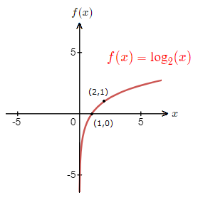
This logarithm graph above is the standard shape for a function f(x) \space {\small{=}} \space {\tt{log}}_a (x) where a > 1.
We can observe the following.
– As x gets smaller towards 0, the graph trends to negative infinity.
– As x gets larger, the graph trends to positive infinity.
– The graph is increasing and doesn’t cross the y-axis.
– The graph will pass through (1,0), and for f(x) \space {\small{=}} \space {\tt{log}}_a (x), will pass through (a,1).
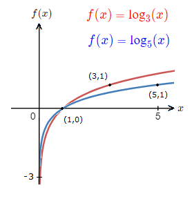
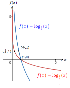
Here is another diagram with 2 other log function graphs for a > 1.
Where we can see how the shape is affected by a varying value of a.
a < 0 < 1
The other case for logarithm graphs is, 0 \lt a \lt 1.We can examine f(x) \space {\small{=}} \space {\tt{log}}_{\frac{1}{2}} (x).
Again obtaining some points on the graph.
f(\frac{1}{4}) \space {\small{=}} \space {\tt{log}}_{\frac{1}{2}} (\frac{1}{4}) \space {\small{=}} \space 2 \space \space \space \space \space \space \space \space \space \space {\footnotesize{( \space (\frac{1}{2})^2 = \frac{1}{4} \space )}}
f(\frac{1}{2}) \space {\small{=}} \space {\tt{log}}_{\frac{1}{2}} (\frac{1}{2}) \space {\small{=}} \space 1 \space \space \space \space \space \space \space \space \space \space {\footnotesize{( \space (\frac{1}{2})^1 = \frac{1}{2} \space )}}
f(1) \space {\small{=}} \space {\tt{log}}_{\frac{1}{2}} (1) \space {\small{=}} \space 0 \space \space \space \space \space \space \space \space \space \space \space {\footnotesize{( \space (\frac{1}{2})^0 = 1 \space )}}
f(2) \space {\small{=}} \space {\tt{log}}_{\frac{1}{2}} (2) \space {\small{=}} \space {\text{-}}1 \space \space \space \space \space \space \space \space \space \space {\footnotesize{( \space (\frac{1}{2})^{{\text{-}}1} = 2 \space )}}
f(4) \space {\small{=}} \space {\tt{log}}_{\frac{1}{2}} (4) \space {\small{=}} \space {\text{-}}2 \space \space \space \space \space \space \space \space \space \space {\footnotesize{( \space (\frac{1}{2})^{{\text{-}}2} = 4 \space )}}
We have found the points (\frac{1}{4},2) , (\frac{1}{2},1) , (1,0) , (2,{\text{-}}1) , (4,{\text{-}}2).
This information can now help in drawing the graph for f(x) \space {\small{=}} \space {\tt{log}}_{\frac{1}{2}} (x).
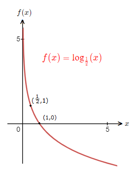
This logarithm graph above is the standard shape for a function f(x) \space {\small{=}} \space {\tt{log}}_a (x) where 0 \lt a \lt 1.
The following can be observed.
– As x gets smaller towards 0, the graph trends to positive infinity.
– As x gets larger, the graph trends to negative infinity.
– The graph is decreasing and doesn’t cross the y-axis.
– The graph will pass through (1,0), and for f(x) \space {\small{=}} \space {\tt{log}}_a (x), will pass through (a,1).
Like before, we can view another diagram with 2 other log function graphs for 0 \lt a \lt 1.
Observing how the graph shape is affected by a varying value of a.
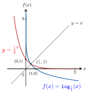
Relationship with the Exponential Function Graph
A logarithmic function is the inverse of its corresponding exponential function.
As such, the graph of the functions are reflected in the line y = x.
The coordinates get swapped around.