Graphs of linear equations can be drawn when the equations are of the form: y = ax + b.
Such as with the example below.
More specifically, the ‘slope intercept’ form of a straight line is the equation: y = {\text{m}}x + c.
Where the letter m represents the slope or gradient of the straight line.
While the letter c represents the point at which the straight line touches the y-axis.
Slope/Gradient of a Straight Line:
We’ll give a brief overview of the gradient of a straight line here, though we will go into it in more detail on the topic in a more concentrated straight line section.The gradient is often written as a fraction but can be a whole number, and describes numerically how steep a straight line is.
The larger the number the gradient m is, the steeper the slope.
Also, the nature of m tells us the slope direction.
A positive gradient is a slope moving upward from left to right. /
While a negative gradient is a slope moving downward from left to right. \
Drawing Graphs of Linear Equations
Examples
(1.1)
Sketch the graph of y = {\large{\frac{5}{3}}}x + 1.
Solution
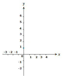
The first step here is to mark a point on the y-axis with the information we have from the linear equation.
The c value is 1,
so we know the straight line will touch the y-axis at (0,1).
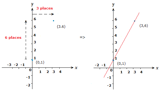
Now we look at the gradient value m, which here is \frac{5}{3}.
Now the gradient as a fraction is \frac{{\text{difference \space in}} \space y}{{\text{difference \space in}} \space x}.
What this means for us here, if that we begin at our starting point of 1 on the y-axis.
Then go 5 points up the y-axis, and 3 points along the x-axis to the right.
Giving us (3,6).
This is the correct slope of the line so the new coordinate we find will be another point on the straight line, thus enabling us to draw the line.
We really only need to know two points on a straight line to be able to make a sketch on a suitable axis.
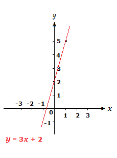
(1.2)
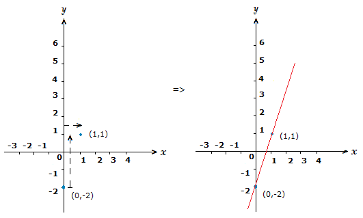
Sketch the graph of y = \space 3x \space {\text{--}} \space 2.
Solution
The coordinate on the y-axis this time will be (-2,0).
For finding our second coordinate using the slope/gradient, we can treat the m value 3 as a fraction, \frac{3}{\scriptsize{1}}.
So like in example (1.1), we go 3 places up the y-axis, and 1 place right along the x-axis.
(1.3)
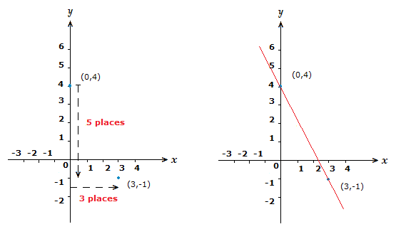
Sketch the graph of y = {\text{-}}{\large{\frac{5}{2}}}x + 4.
Solution
So we can see that the coordinate on the y-axis is (4,0).
But we have a negative value for m this time.
This means that in finding the second coordinate of the straight line using the slope, we will initially move down the y-axis, but still moving right along the x-axis.
That’s the thing to remember with negative m values, y places move downward, but x places still move right, as they also do when m is positive.
Drawing Graphs of Linear Equations,
Alternative Method
When attempting to graph a linear equation, an alternative approach is to work out several points on the line, plot them and then connect them with a straight line.
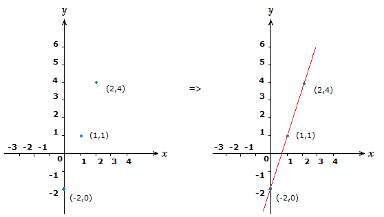
If we look again at the linear equation in example (1.2).
We can plug in some x values to obtain some points.
x = 0 => y = 3(0) \space {\text{--}} \space 2 \space = \space {\text{-}}2 (0,–2)
x = 1 => y = 3(1) \space {\text{--}} \space 2 \space = \space 1 (1,1)
x = 2 => y = 3(2) \space {\text{--}} \space 2 \space = \space 4 (2,4)
These 3 points will be sufficient to plot and thus draw the correct straight line.